Anomaly Detection in Electricity Consumption

Important facts:

Anomaly detection is a very important and active business metric for various fields. A technique that is used to identify the unusual patterns that are not in sync with the expectations.
It has many applications in business-like health (detecting health discrepancies), cybersecurity(intrusions), electricity (huge and sudden surges), finances (fraud detection), manufacturing (fault detection), etc. This shows that there is more to anomaly detection in everyday life and important concepts to be looked at.
The data science application in anomaly Detection combines multiple concepts like classification, regression, and clustering.

Business Case

Electricity consumption of society has been increasing steadily day by day and it has become important for generators and suppliers to meet the demand and be vary of the sudden increase or surges in their distribution.
Typically, there is more energy consumption than necessary due to various supply losses, malfunctioning equipment, incorrectly configured systems, and inappropriate operating procedures. Therefore, it is very important to have a quick response and reliable fault detection to ensure they met the demand, have a breakless service, and save energy.
Electricity supply can be having point, contextual or collective anomalies. The electricity anomalies could fall into either of the three categories. Sudden surges at a locality or on holidays or an activity taking at a place etc.
These anomalies could follow a pattern like high electricity usage in summer or sudden spike due to wedding activity (wedding season) or point anomaly (for example, when someone starts mining a bitcoin – which takes a lot of power)
Detecting this helps the stakeholders to plan for additional supply, curb the untoward electricity usage, and leakages, and save a lot of money and energy for all stakeholders.

Steps Involved:

Initial Thinking

Identifying anomalies is a tricky task as the data doesn’t always tell what it is. It could just an outlier or it was an anomaly. The set of anomalies/outliers will be very few and hence the data is imbalanced for any algorithm to learn. Especially in electricity anomaly detection, there are too many factors like weekend, office area, holiday area, etc.
How to capture an anomaly then? My initial ideas were to use the time series data and predict the values based on various engineered features and calculate the residue. When the residue crosses the excess level mark that as an anomaly. This level can be decided based on various factors like a combination of time of duration, temperature, day of activity, etc. Then compare all the residues and mark the residues with exceeding level as anomalies. But before this, I have to remove all the outliers captured in the data.
Another idea that popped at me was finding the nearest neighbors and predict the values based on various features. Once the value predicted for a day based on nearest neighbors is different than the usual mark them unusual and consider the other factors to whether mark them as anomalies or not. Using KNN will help here. But defining the number of nearest neighbors and the relationship between some neighbors might become difficult in the starting as there could too many correlations.
An important point to remember: Outliers are observations that are distant from the mean or location of a distribution. However, they don’t necessarily represent abnormal behavior or behavior generated by a different process. On the other hand, anomalies are data patterns that are generated by different processes.

Technologies Used

Python
Pandas
Numpy
Plotly
Scikit-Learn
Boosting
XGBoost
Isolation Forest

SKILLS

EDA
Time Series Analysis
Supervised ML
Statistics
Data Visualization

Data Acquisition

Data downloaded from Scheider Electric.
The data consisted of 5 CSV files.
- Training data with timestamp and values of electric units for respective meter ids.
- Weather data with a timestamp, temperature, site ids, and distance.
- Holidays CSV files consisted of Date, type of holiday, and site_ids.
- Metadata CSV file consisted of site Id, meter_id, Meter Description, units, surface, and activity.
- The submission file had the true values of whether it is an anomaly or not.

Preprocessing – Data formatting and Munging

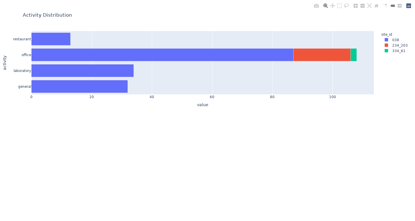
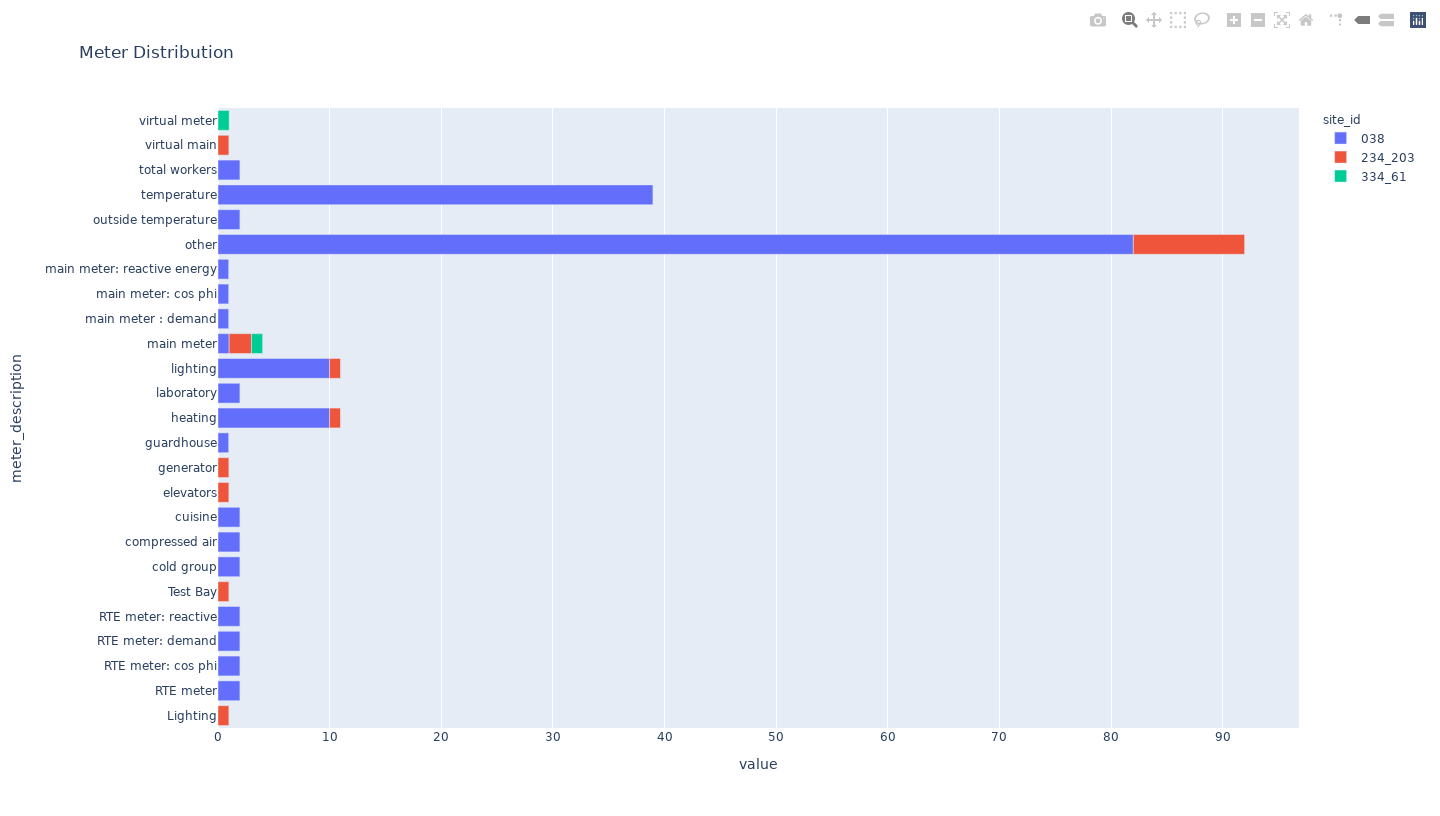
The given data is for three sites (Site 38, 234_203, 334_16) and more than 20 meter_ids. The data covers more than 4+ years of data. The given data also covers various kinds of activities like restaurants, offices, laboratories, general. The meter ids have even more vast distribution across 3 sites covering various electricity usage like elevators, generators, compressed air, etc.
From exploring the above data, it was clear that a lot of data is missing between various data tables. Not all site ids have been mentioned for the respective meter ids.
- The data is skewed towards one site.
- The presence of wrong data in electric Units are present
- Metadata is filled with many unknowns
- Weather datatable doesn’t contain data for site 234_203

Feature Selection & Engineering

Considering the subject (electric unit values prediction) and the data given, I started wondering what factors lead to electricity consumption for a place or activity. For a house, it could outside temperature, people staying at home on a holiday and for a office outside temperature, full staff, hectic day or long-day etc.
I started to extract all the features like a year, month, day, hour, sin, and cos values of month & day. Whether it is a working day or not, whether it is a weekend or not, day of the year, night, reset hour, the temperature outside, mean temperature across the day, mean temperature across the month, is it a holiday, etc.
These are some of the features that occurred to my mind and some based on exploration of the internet.
Now the important question is how many of these factors are important and what weight they carry on.
Before moving on to modeling, I wanted to check how the electric unit values are spread across 4 years.
- Below is the representation of weekday(blue) and weekend value(green) for sites 334 and 234.
- We can see there are few spikes here and there. We don’t know whether they are anomalies are not. But definitely, they are not outliers.
- Also, we can see that the green values are not high enough. This is due, site 334_61 & 234_203 is predominately office activity and on weekends they are assumed to be non-functioning.

</html>

Features Code

```python# def basic_feature_engineering(df): night_hours = {20:0,21:1,22:2,23:3,0:4,1:5,2:6,3:7,4:8,5:9,6:10} day_hours = dict([(h,i) for i,h in enumerate(range(7,20))]) df['year'] = pd.DatetimeIndex(df['Timestamp']).year df['month'] = pd.DatetimeIndex(df['Timestamp']).month df['month_sin'] = np.sin(df['month']*2*pi/12) df['month_cos'] = np.cos(df['month']*2*pi/12) df['day'] = pd.DatetimeIndex(df['Timestamp']).day df['hour'] = pd.DatetimeIndex(df['Timestamp']).hour df['day_sin'] = np.sin(df['day']*2*pi/30) df['day_cos'] = np.cos(df['day']*2*pi/30) #df['day_of_week'] = pd.DatetimeIndex(df['Timestamp']).weekday_name df['day_of_week'] = pd.DatetimeIndex(df['Timestamp']).day_name() df['working_day'] = (df['day_of_week']!= 'Saturday' )&(df['day_of_week']!= 'Sunday' ) df['weekofyear'] = pd.DatetimeIndex(df['Timestamp']).weekofyear df['weekofyear_sin'] = np.sin(df['weekofyear']*2*pi/52) df['weekofyear_cos'] = np.cos(df['weekofyear']*2*pi/52) df['dayofyear'] = pd.DatetimeIndex(df['Timestamp']).dayofyear df['dayofyear_sin'] = np.sin(df['dayofyear']*2*pi/365) df['dayofyear_cos'] = np.cos(df['dayofyear']*2*pi/365) df['hour_sin'] = np.sin(df['hour']*2*pi/24) df['hour_cos'] = np.cos(df['hour']*2*pi/24) df.loc[(((df['hour']>=20 )&(df['hour']<= 23 ))|((df['hour']>=0 )&(df['hour']< 7 ))),'night']= True df['night'].fillna(False,inplace = True) df.loc[df['night']==True,'reset_hour']= df.loc[df['night']==True,'hour'].apply(lambda x: night_hours[x] ) df.loc[df['night']==False,'reset_hour']= df.loc[df['night']==False,'hour'].apply(lambda x: day_hours[x] ) df.loc[(((df['hour']>=22 )&(df['hour']<= 23 ))|((df['hour']>=0 )&(df['hour']< 7 ))),'time_of_day']= 0 df.loc[(((df['hour']>=7 )&(df['hour']< 10 ))|((df['hour']>=18 )&(df['hour']< 22 ))),'time_of_day']= 1 df.loc[(((df['hour']>=10 )&(df['hour']< 18 ))),'time_of_day']= 2 df['minute'] = pd.DatetimeIndex(df['Timestamp']).minute return df def fea_day(df,weather_mod): df = basic_feature_engineering(df) df.dropna(subset = ['Values'], inplace = True) df = pd.merge(df,weather_mod[['year','month','day','hour','Temperature']], how='left', on = ['year','month','day','hour']) df = df.join(df[['year','month','day','Temperature']].groupby(['year','month','day']).mean(), on = ['year','month','day'],rsuffix = '_mean_date') df['Temperature_sq']=df['Temperature']**2 df['night'] = df['night'].astype(int) df = df.join(df[['year','month','day','night','Temperature']].groupby(['year','month','day','night']).mean(), on = ['year','month','day','night'],rsuffix = '_mean_time_of_day') df = df.join(holidays_mod[['year','month','day','is_holiday']].set_index(['year','month','day']), on = ['year','month','day']) df.is_holiday.fillna(False, inplace = True) df['is_holiday'] = df['is_holiday'].astype(int) df['is_abnormal'] = False df['high_temp'] = df['Temperature_mean_date']>17 df.loc[(df.Timestamp>'2015-08-09')&(df.Timestamp<'2015-08-15'),'is_holiday']= True df.loc[((df['working_day']==True)&(df['high_temp']==True)&(df['is_holiday']==False)),'model_num'] = 1 df.loc[((df['working_day']==True)&(df['high_temp']==False)&(df['is_holiday']==False)),'model_num'] = 2 df.loc[((df['working_day']==False)&(df['high_temp']==False)&(df['is_holiday']==False)),'model_num'] = 3 df.loc[((df['working_day']==False)&(df['high_temp']==True)&(df['is_holiday']==False)),'model_num'] = 4 df.loc[((df['day_of_week']=='Saturday')| (df['day_of_week']=='Sunday') | (df['is_holiday']==True)),'model_num'] = 5 df['model_num'].fillna(0,inplace = True) df['working_day'] = df['working_day'].astype(int) df['is_holiday'] = df['is_holiday'].astype(int) return df ```

Model Selection & Training

As the electricity data is time-series data, I decided to use regression-based supervised learning model (XGBoost) to predict the future values based on past values and extracted feature engineering. The features I used are as follows
- Rolling mean, moving average, temperature, and other features like a year, month, weekend, weekday, cos and sin feature of day and month, etc.
- Choosing XGBoost was an active choice as it has been the most efficient gradient boosting algorithm. It produces prediction by combining an ensemble of weak predictors.
- To avoid overfitting, I used cross validation to split the train and test data sets
- Since I am using regression for prediction, I used RMSE metric to calculate the error.
We have seen above that the weekend and weekday consumption values are a lot different and the same model cannot be used. Hence I decided to use the Isolation forest model for weekend prediction. While using isolation forest, I tried using the normalizaed 24 hours values rather than direct values because, weekend consumption appeared to be level distributed and didn’t want a prediction solely on some factors.
For weekend anomaly detection, I borrowed some features from an github solution.
- The features he has selected as follows. (I felt these are extensive and best features for an isolation forest algorithm and hence I couldn’t perform any better than this)
  - The power values of each hour are extracted as features.
  - Temperature
  - Power value after 9:00am as its a weekend and the consumption values after a bit of morning project the real consumption.
  - Kullback-Leibler Divergence: Measure of how one probability distribution diverges from the empirical distribution. We calculate the mean value of power usage of each hour as the empirical distribution, then calculate the KL divergence of each weekend 24-hr power usage with the empirical distribution.
  - The hour of daily power values’ peak because if peak occurs later in the day suddenly, it could be an anomaly.
- Isolation forest is an effective unsupervised algorithm with a small requirement.
- The way this algorithm works is that first it build isolation trees by randomly selecting features and then starts splitting the data based on features’ break points. Then anomalies are detected as instances which have short average path lengths on the isolation trees.
But the case is not over yet. We predicted the consumption values and now have to detect the anomalies
- I defined an anomaly if the predicted error exceeds a defined rule-based threshold.
- Here I plotted the error values after converting a distribution (gaussian) by resampling with respect to day with mean values and identifying those error values which fall in 2 sigma level.
- The extreme large errors are labelled as anomalies.
The predicted anomalies are visuaized below (light shaded straight lines belongs to weekdays & dark shaded straight lines belong to weekend)
- For site 334

</html>

For site 234

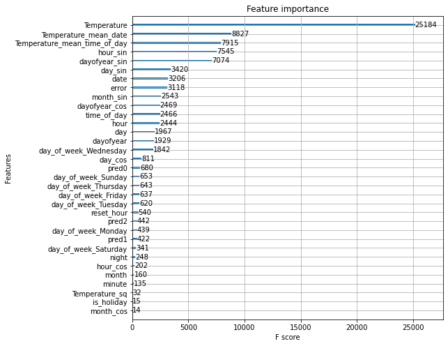
#### Feature Importance from the model:

##### SITE 234: Feature Importance for site 234

##### SITE 334: Feature Importance for site 334

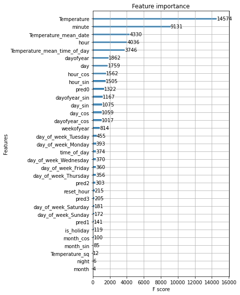
From the above feature importance images it is clear that the temperature, minutes, day and hours play an important role in predicting the values of electric consumption.

Future Work and Scope

This work can be further improved using a more rule-based approach to decide the right anomalies for each site and meter id. Using PCA and more feature engineering can give us more accurate predictions and then using rule-based hand-holding can help us achieving in more accuracy.
There is a lot of research going on in detecting anomalies in various sectors. The neural networks, GANs (novel unsupervised learning methods) are becoming more efficient in identifying anomalies. These methods can be very well be used to tabular data as well.

MY LEARNINGS:

My biggest takeaway from this project is anomaly pattern detection need subject matter expertise more than any other data science field.
This is one the important and practical field with very high stakes in the real world.
Combining time series and anomaly detection increases the stakes even more higher in a business.
It is very important to define the rules to fix a threshold to identify the anomaly.
Having more anomaly alerts is better than having less.
Isolation forest an unsupervised algorithm is very helpful in predicting with short average path lengths and also compute with low linear time complexity with very small memory requirement.
Using RAPIDS AI to implement XGBoost using GPU. Wasn’t completely successful. Need to check more

What I tried and couldn’t achieve

The data had more than a 1million rows for some sites. I wasn’t able to figure out a way to use GPU to train on site specific data. I was able to perform only on meter id specific.
Need to figure out GPU based training and incorporate more data for training thereby getting getting more accurate anomalies.