This is from a kaggle competition, where I wanted to participated and apply my learnings in forecasting methods. In this 1st part post, I am exploring the data with various visualization and trying to understand the dataset.
Business case
- It is very important for a large store to forecast the required products for their store to have enough inventory in their store. It is even more important for a company which has multiple chain across states, countries to have a forecast for 28, 60 days and distribute the inventory based upon the need accordingly across the stores. Forecasting for an item, for a store, for a state depends not just on the people, but also various factors like weather, needs and necessities and extraneous situation like pandemic. The best example was the stock out paper towel and bathroom issues during the initial stages of lockdown (March, April). An inaccurate forecast results in actual opportunity cost and overall revenue loss to the company. So, it is very important for the company to forecast it needs and inventory properly.
- By using forecasting methods like Naïve Bayes, moving average, exponential smoothing methods, we can forecast for singular products, but when dealing with larger overall number of products, these methods do not serve much help. Using gradient boosting methods, I created a forecasting model for 28-100 days. We can use this model to forecast overall products for a store, state but not for singular products.
- In the below data exploration, I try to forecast inventory on the overall products for a store for 100 days based upon the data of previous 2 years. This model can take in various parameters according to the needs and tastes of local people and other conditions like SNAP, local festivals and other conditions. With the help of this model, we can forecast the product inventory up to certain accuracy.
Table of Contents
- File Descriptions
- Technologies Used
- Structure
- EDA
- Modelling and Hyperparameter Tuning
- Evaluation & Prediction
- Future Work
Problem Description in depth
The data contains hierarchical sales data, made available by Walmart, starting at the item level and aggregating to that of departments, product categories, stores in three geographical areas of the US: California, Texas, and Wisconsin. This data contains item levels, department levels, product category level, store details for 5 years. This gives scope for more than 40k time series levels. We have to forecast for all the products depending upon the need and necessity within our computing resources.
File Descriptions
- Data: Folder containing all data files. It has three main files to work with
- Calendar: This data file contains the date, respective week ids, festival events and SNAP days in three states
- The festivals vary from state to state and they have also been divided into two event types
- Prices: This data file contains the id of the product, its prices on that particular day and id of the week.
- Sales: This the main data file. It contains items id and their sale on each day from 01/29/2011 to 05/22/2016.
- Calendar: This data file contains the date, respective week ids, festival events and SNAP days in three states
Technologies Used
- Python
- Pandas
- Numpy
- Matplotlib
- Seaborn
- Plotly
- Scikit-Learn
- LightGBM
- XGBoost
- Pytorch
SKILLS
- EDA
- Time Series Analysis
- Supervised ML
- Statistics
- Data Visualization
Data Description
- This data contains sales data of 3 states.
- Each state contains in total 10 of stores.
- These 10 stores sold nearly 3049 products in each store.
- That gives us the data for 30490 products across all the stores.
- The products sold in these 10 stores have been divided into 7 categories i.e., Hobbies 1, Hobbies2, Household 1, Household2, Foods 1, Foods 2, Foods 3.
- For example: TX(3 stores) –> Stores –> Categories(Hobbies, foods, household) –> Departments –> Items
- This data leads us to number of time series aggregated across various combinations.
- Unit sales of all products aggregated for all states and stores – 1
- Unit sales of all products aggregated for each state – 3 [ California, Texas, Wisconsin]
- Unit sales of all products aggregated for each store – 10
- Unit sales of all products, aggregated for each category – 3 [Hobbies, Household, Foods]
- Unit sales of all products, aggregated for each department – 7 [ 3 categories – 7 department]
- Unit sales of all products, aggregated for each state and category – 9
- Unit sales of all products, aggregated for each state and department – 3x7 = 21
- Unit sales of all products, aggregated for each store and category – 3x10 = 30
- Unit sales of all products, aggregated for each store and department – 7x10 = 70
- Unit sale of a product x, aggregated for all stores/ states = 3049
- Unit sale of product x, aggregated for each state = 3049x3 = 9147
- Unit sale of product x, aggregated for each store = 3049x10 = 30490
- The data is from 01/29/2011 to 05/22/2016.
- The forecast requested for dates 05/23/2016 – 06/19/2016
- The hierarchical nature of the datasets makes it possible to do a top-down or bottom-up approach.
- There are around 34 events mentioned by Walmart sales data.
- Having so many levels of hierarchical data, working the time series data will be requiring good computing resources. This need for more computing resources increases with the need of higher accuracy and increase in hierarchical level needed.
EDA and Pre-processing
Exploration
Total Products sold across the States
- I going to explore the data as various hierarchical level.
- Looking at the data how many total products are sold across the states
-
The above figure shows the number of products sold in three states across 5 years. The difference between CA and other two states TX, WI is significant. This can be explained by the fact that the population in CA is way more than the other two states.
-
Now lets see which products are sold and their share in the three states
This shows that the foods products are sold more across all states and hobbies products are sold the least. So an insight which can be drawn here is that a company should be more careful in forecasting and having inventory of the food products.
Total Products sold across the Stores
- Now lets look at total products sold by each store in the three states
Here again we see that CA stores sold more products in the last 5 years combined than most other state stores. It is pretty clear now that the CA needs more products and better forecasting in order to serve customers properly as this state has more business proposition than other states compared
Mean Sales of Products sold across the Stores
- Now lets look at the mean sales with a rolling mean of 90 over a day in each store
The above graphs shows the lowest sales, mean sales and median sales of all products combined across all the ten stores. CA1, CA3 stores appeared to be selling more products. With earlier inference of food products being sold high in all states and stores, we can safely assume that these stores might be located in highly densely populated areas and these are serving more people and have high business turnovers. So these store might require highera attention in the needs of product distribution and diversification.
After having started with initial exploration, let’s go a bit deeper. The main variables in this whole dataset have been unit sales(demand), price, items_ids,etc.
EXPLORING PRODUCTS AND PRICES OF CATEGORIES
Exploring the number of products in category
The above graph pretty much explains the insights. Number of products in each category products in across all the states. So we have access to symmetrical data for the three states.
Mean Prices across departments
Here we explore the mean prices of all products across the three different states. As seen earlier the hobbies products have been sold less, and we can see one of the reason here being the prices on the higher side. One interesting observation is that the mean prices of the all products combined appeared to be same across the three state. Geographical distance didn’t affect the price range of products.
Price Distribution
After exploring the number of products, mean prices across departments, we will be exploring the price distributions of the total 3049 item_ids. We can see the food products sell prices are less than $20 and mostly concentrated less $7. Hobbies products sell prices are consistent across all the stores and states, whereas Household products sell prices are consistent across CA but have some outliers in TX_1, WI_2, WI_3 stores. Apart from that, the distribution of all the products has been similar across all the stores. This infers that prices are consistent across the geography.
Product Sales across the three states
This visual gives me more clear insights into what kind of products are being sold highest and in which states. Seems to be FOODS_3 are highest selling and HOBBIES_2 are lowest selling. A deep look in the characterization of the products will give us even more insights. As for this data we have only item_ids with numbers. Hence we are not concerned with that for now.
Category - Department - products sales across the state
FOODS_3 department products are sold more than 50% in CA than that of other the two states. Even Household_1 and Household_2 products appeared to be sold more than 50% in CA compared to TX & WI. All products in CA are sold more compared to TX & WI.
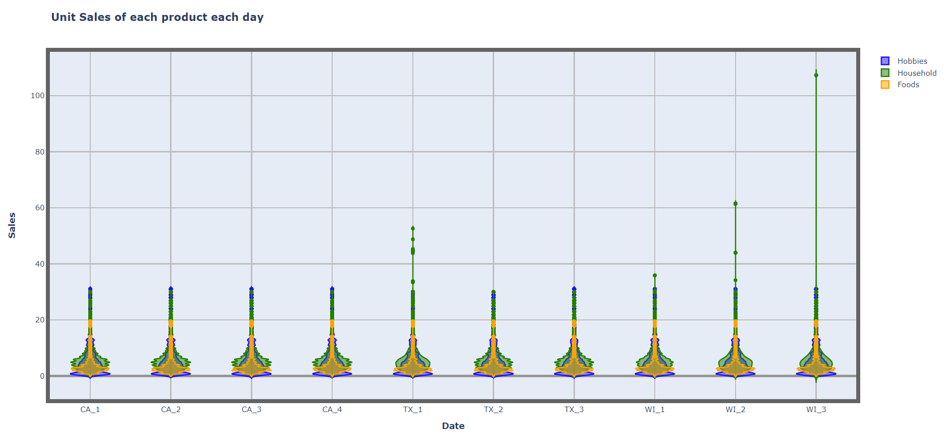
UNIT SALES OF EACH CATEGORIES IN EACH STORE
Exploring with another visual, where we infer that the foods continue to be the highest selling products across all the stores and then comes the household products. CA_3 store has the highest selling of all products when compared with other stores. We could infer that this could be the largest store in CA or this could be the place with the highest population. The second selling store appears to be CA_1 for foods, but CA_2 for household and TX_2 is also close by.